Tensor Parallelism and Sequence Parallelism: Detailed Analysis
Table of Contents
This post explains how tensor model parallelism and sequence parallelism work especially on attention layer, and how they are different.
Backgrounds #
Attention Layer #

T number of tokens. d_attn is config.embed_dim // config.num_attention_heads Bold boxes are model parameters, while others are temporarily created tensors.
All the other terms are borrowed from HuggingFace Transformers OPT config. Implementation of computing attention:
class OPTAttention(nn.Module):
    def __init__(self, ...):
        ...
        self.k_proj = nn.Linear(self.embed_dim, self.embed_dim, bias=self.enable_bias)
        self.v_proj = nn.Linear(self.embed_dim, self.embed_dim, bias=self.enable_bias)
        self.q_proj = nn.Linear(self.embed_dim, self.embed_dim, bias=self.enable_bias)
        self.out_proj = nn.Linear(self.embed_dim, self.embed_dim, bias=self.enable_bias)

    def forward(...);
        # hidden states is an input tenor of Attention layer
        # Calculate Q, K, and V with linear projections to the input
        query_states = self.q_proj(hidden_states) # apply self._shape() later
        key_states = self.k_proj(hidden_states) # apply self._shape() later
        value_states = self.v_proj(hidden_states) # apply self._shape() later

        # QK^T
        attn_weights = torch.bmm(query_states, key_states.transpose(1, 2))

        # apply mask if exists

        # softmax
        attn_weights = nn.functional.softmax(attn_weights, ...)

        # dropout
        attn_probs = nn.functional.dropout(attn_weights, ...)

        # multiply by V
        attn_output = torch.bmm(attn_probs, value_states)

        ...

        # final linear
        attn_output = self.out_proj(attn_output)
$$\text{Attention}(Q, K, V)=\text{softmax}(\frac{QK^T}{\sqrt{d^k}})V$$
Attention is to calculate the probability of the next token, given all the previous tokens in the context.
How Calculating Attention in Training and Inference is Different? #
Calculating attention itself is the same ($\text{Attention}(Q, K, V)=\text{softmax}((QK^T)/\sqrt{d^k})V$).
Then how calculating multiple tokens can be parallelized in training and prefill stage of inference, while decode stage in inference can’t?
This is because, for each token in training and prefill, all previous tokens are already given as its context.
In training or prefill stage, there is no KV cache; thus K and V for every tokens need to be computed.
For example, a-th token needs to compute K and V for all [0...a-1]-th tokens, and its context length Ta is a, while b-th token has context length is b.
If a < b, it is true that we can utilize K and V for a-th token as cache during calculating K and V of b-th token; but it adds dependecy between token computation, so it is typical to just utilize massive parallelization of accelerators and independently calculate each tokens’ K and V in parallel even though it introduces a lot of redundancy.
For decode stage in inference, on the other hand, generates one token per iteration, and K and V for previous tokens are already computed and stored as a cache; thus redundant computation is unncessary. But, we do not know which token will be chosen for the current location, therefore we cannot prefetch K and V calculation for all future tokens.
Difference in Sequence, Token, and Batch #
To understand differences between tensor parallelism and sequence parallelism, you need to know first what are sequence and token. Sequence is an input text, which consists of multiple tokens. Even in a single batch, an input sequence includes several tokens which can be parallelized via sequence parallelism.
This can be applied in training, or prefill stage of inference. For decode stage of inference, only one token is given per iteration; unless multiple requests are batched, sequence parallelism cannot be applied in decode stage.
Note that all examples in this post uses batch size 1. the dimension of hidden_states :[T, embed_dim] is actually [1, T, embed_dim], where batch size is 1, and token size is T.
For input with dimension [B, T, embed_dim]:
- Data parallelism with DP degree
d: input dim per GPU will be[B/d, T, embed_dim] - Sequence parallelism with SP degree
s: input dim per GPU will be[B, T/s, embed_dim]
Both DP and SP can be applied together, making 2D parallelism for input and 4D parallelism for the entire parallel execution (data parallelism, sequence parallelism, pipeline model parallelism, and tensor model parallelism).
Tensor Model Parallelism #
Tensor model parallelism splits and distributes model parameters into multiple GPUs, thus their FLOPs are divided.
Model parameters in attention are included in q_proj, k_proj, v_proj, and out_proj.
Based on their location in matrix multiplication, they are sliced vertically (ColumnParallelLinear) or horizontally (RowParallelLinear).
This 1D tensor model parallelism is first introduced by Megatron-LM 1 and widely adopted in both training and inference, including HuggingFace ML serving system TGI.
Implementation of OPTAttention in TGI supports tensor parallelism as:
class OPTAttention(nn.Module):
    def __init__(self, ...):
        self.q_proj = TensorParallelColumnLinear.load(
            config, prefix=f"{prefix}.q_proj", weights=weights, bias=bias
        )
        self.k_proj = TensorParallelColumnLinear.load(
            config, prefix=f"{prefix}.k_proj", weights=weights, bias=bias
        )
        self.v_proj = TensorParallelColumnLinear.load(
            config, prefix=f"{prefix}.v_proj", weights=weights, bias=bias
        )
        self.out_proj = TensorParallelRowLinear.load(
            config, prefix=f"{prefix}.out_proj", weights=weights, bias=bias
        )
According to the implementation, q_proj, k_proj, v_proj are column parallelized, and out_proj is row parallelized. Let’s see why.
In calculating Q, K, and V, tensor parallelism is typically done by splitting the number of heads with the number of GPUs. For example, OPT-175b model has 96 heads in each decoder layer. If we use tensor parallelism with 8 GPUs, then each GPU computes 12 heads, instead of all 96 heads. Example of vllm:
class QKVParallelLinear(ColumnParallelLinear):
    def __init__(self, ...):
        ...

        # Divide the weight matrix along the last dimension.
        tp_size = get_tensor_model_parallel_world_size()
        self.num_heads = divide(self.total_num_heads, tp_size)
        if tp_size >= self.total_num_kv_heads:
            self.num_kv_heads = 1
            self.num_kv_head_replicas = divide(tp_size,
                                               self.total_num_kv_heads)
        else:
            self.num_kv_heads = divide(self.total_num_kv_heads, tp_size)
            self.num_kv_head_replicas = 1
Because tensors per head are assigned in columns, it is natural to use ColumnParallelLinear to parallelize Q, K, and V linear projection matrices.
For out_proj, it is the last matrix to be multiplied; and to make dimension suitable for matrix multiplication, it is split in row-wise.
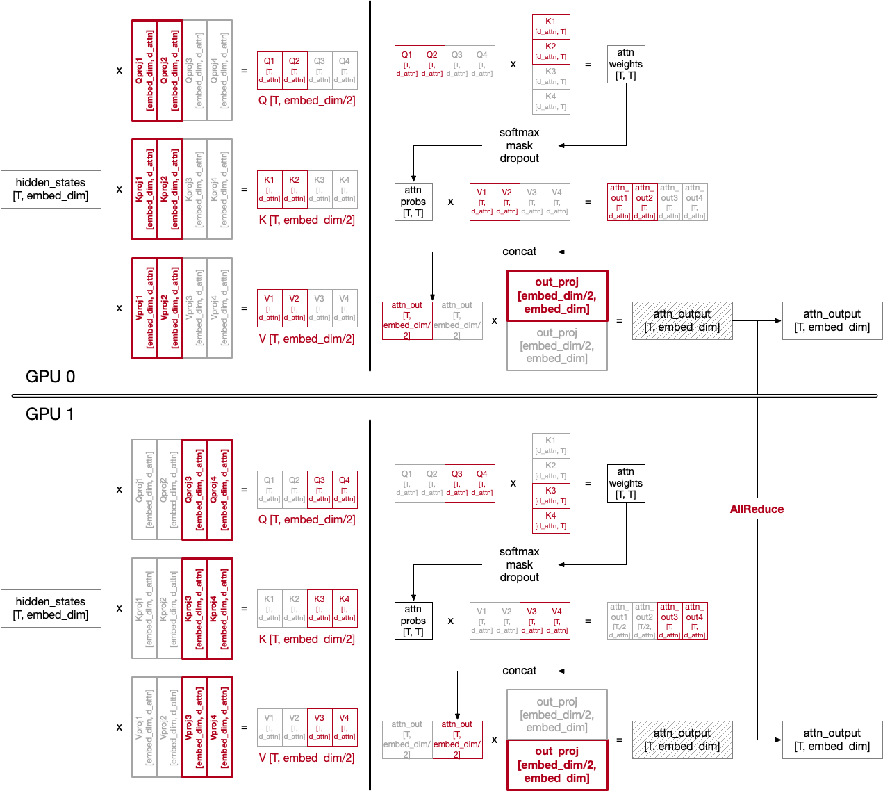
attn_output, although both GPUs have the output with correct dimension, their computation result is distributed; hence, call all_reduce on attn_output. It is implemented in RowParallelLinear’s forward():
class TensorParallelRowLinear(SuperLayer):
    ...
    def forward(self, input: torch.Tensor, reduce: bool = True) -> torch.Tensor:
        out = super().forward(input)
        if self.process_group.size() > 1 and reduce:
            torch.distributed.all_reduce(out, group=self.process_group)
        return out
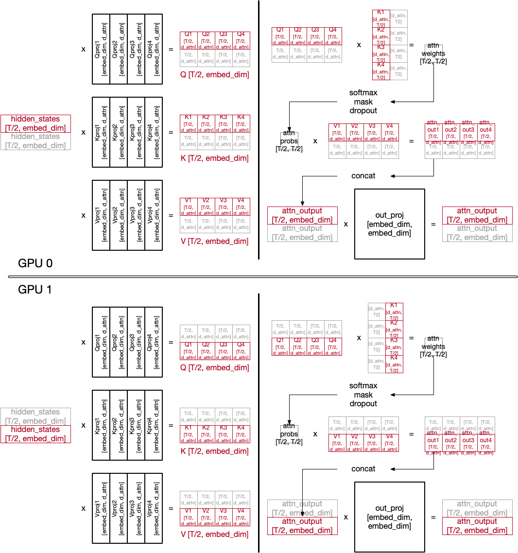
Sequence Parallelism #
Unlike tensor model parallelism, sequence parallelism splits input data (hidden_states).
Data parallelism does also split input to mini-batch, but sequence parallelism has an advantage that it can even split a single batch. It introduced in several papers 2 3 4.
Sequence parallelism parallelizes token processing in multiple GPUs. As it partitions inputs, each GPU has the entire copy of model parameters (of course, if tensor model parallelism is applied together, model parameters are partitioned by TP).
pad_token to make their number of token the same to the largest one.
Not the entire forward pass is drawn, as we are focusing on attention layer.
In forward, input tensor hidden_states is just partitioned but needs to be gathered in backward.
After the last layer, decoder-based models has ln_f LayerNorm layer, which requires the whole output. Before calling it, outputs are gathered.
Here is an example of ColossalAI’s implementation of GPT:
def gpt2_model_forward(...):
    ...
    input_embeds = self.wte(input_ids)
    position_embeds = self.wpe(position_ids)
    hidden_states = input_embeds + position_embeds
    hidden_states = self.drop(hidden_states)
    ...

    if enable_sequence_parallelism:
        hidden_staes = split_forward_gather_backward(...)

    for i in range(num_hidden_layers):
        self.h[i](hidden_states, ...)

    if enable_sequence_parallelism:
        hidden_states = gather_forward_split_backward(...)

    hidden_states = self.ln_f(hidden_states)
    ...
Note that, even if the number of tokens are evenly distributed, the amount of computation per worker is different. This is because of how attention is computed with key and value. Basically, attention is, given the context with all previous tokens, to calculate the probability of the next token.
Therefore, calculating attention for later tokens needs to consider more number of previous tokens, like the figure below:
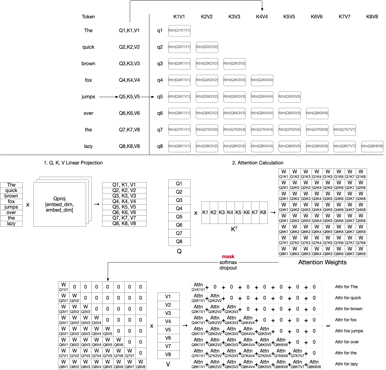
With no sequence parallelism, all Q, K, V calculations and attentions can be done together in a single GPU. With sequence parallelism, however, Q, K, and V are distributed and a way of efficient computing distribution is needed. For example, if we simply distribute each token to workers (e.g. The to worker 1, quick to worker 2, brown to worker 3, …), they have imbalanced amount of calculation, leading to inefficiency (later tokens have more amount of computation). Therefore, papers for sequence parallelism try to handle this imbalance problem in various ways.
Ring Self-Attention (RSA) 2 #
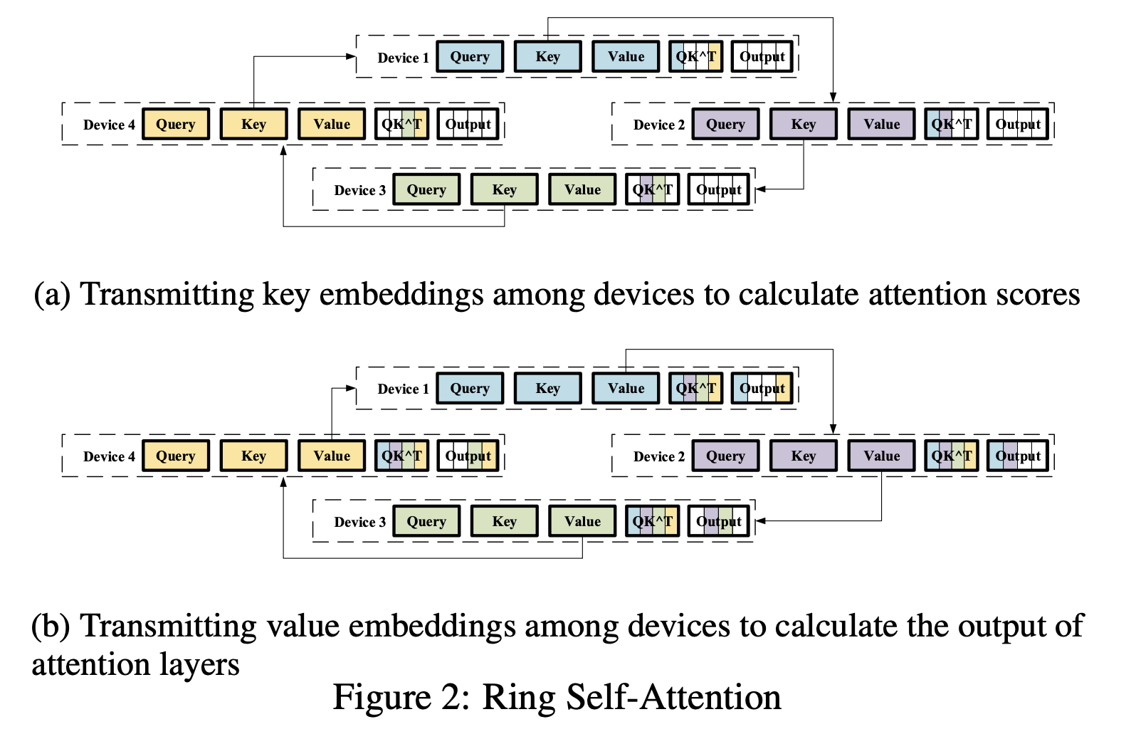
As you can see in the matrix of KV for each query, there are a lot of redundant computation (for key and value for the first The, it is computed 8 times, in every workers).
RSA instead adopts allgather style approach to minimize redundant computation.
Each worker n only computes Q, K, and V for its own token q_n, k_n, v_n.
Let’s see an example with 4 workers for simplicity.
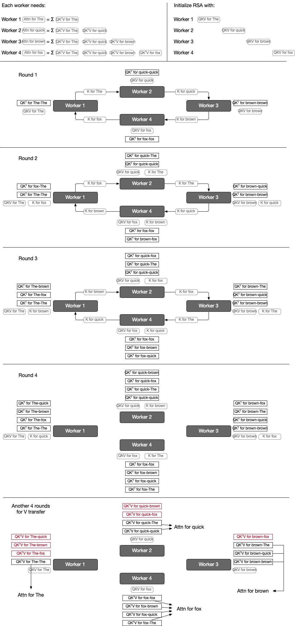
At round 1, computing $QK^T$ for its own token and transferring its key to the next work happens together. At the next round, compute partial attention score ($QK^T$) using its own query and given key ($QK^T$ for T1-T2 means calculating $QK^T$ for query token T1 and key token T2). At the last round of K transfer, all workers have all $QK^T$ for every token’s key and its own query.
RSA goes through another set of rounds to transfer V matrices too, and after the second round each worker will have $QK^TV$ for all pair of its own query token and all key tokens; now they can calculate attention for their own query.
Note that attention only looks at the previous context, partial attentions calculated for future KV are discarded (highlighted as red).
For example, worker 3 needs attn for brown, which can be calculated by summing partial attention score of The, quick, and brown, utilizes computed $QK^TV$s for brown-The, brown-quick, and brown-brown.
A clear drawback is that it needs too many communication rounds (2(n-1)), and computations cannot be fused.
At each round, a worker computes $QK$ or $SV$ for one key and value, similarly to decoding. This cannot fully saturate the GPU cores and leads to underutilization.
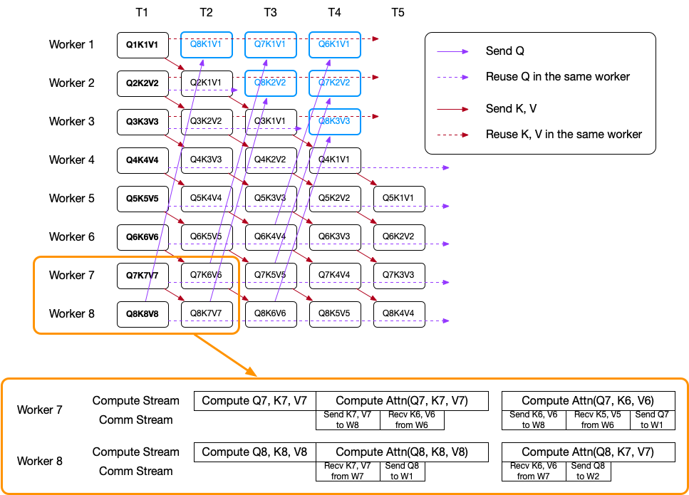
DistAttention 4 #
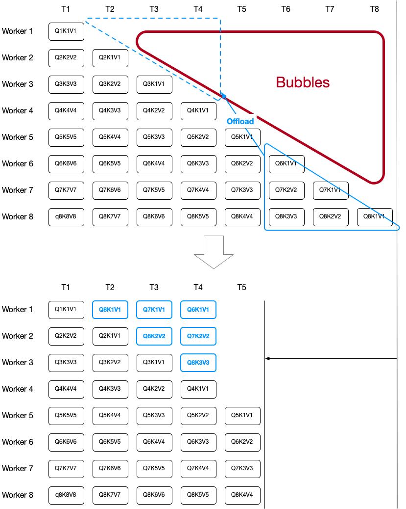
DistAttention completely removes redundant computation and offloads some computation to balance the amount of attention computation across workers. This offloading is quite clever, since it still doesn’t have to compute any Q, K, V redundantly.
-
Efficient Large-scale Language Model Training on GPU Clusters using Megatron-LM ↩︎
-
Sequence Parallelism: Long Sequence Training from System Perspective ↩︎ ↩︎
-
Reducing Activation Recomputation in Large Transformer Models ↩︎
-
LightSeq: Sequence Level Parallelism for Distributed Training of Long Context Transformers ↩︎ ↩︎