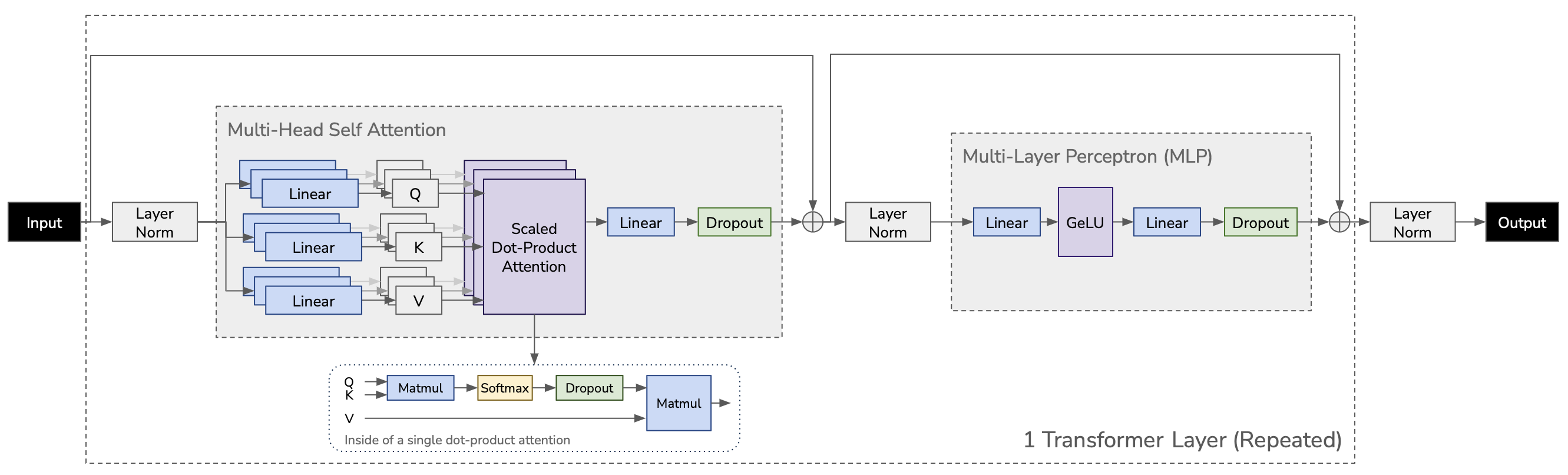
We exploit the inherent parallelism in the multi-head attention operation to partition the self-attention block (shown in Figure 5b). The key (K), Query (Q), and value (V) matrices can be partitioned in a column-parallel fashion. The output linear layer can then directly operate on the partitioned output of the attention operation (weight matrix partitioned across rows).

Deepak Narayanan et al, Efficient large-scale language model training on GPU clusters using megatron-LM, SC'21

This post analyzes how we can parallelize multi-head attentions, which is a type of tensor-parallelism, but more efficiently without heavy communication like traditional intra-layer parallelisms have, which ZeRO ¹ stated so in Section VII-C: MP incurs significantly higher communication compared to ZeRO-DP.

This post in inspired from the following posts ².

In the transformer architecture, multiple attention heads exist together in each transformer layer, i.e. 16 heads in GPT-2 medium. They are independent and linear projections (matmul) in multi-head self attention can be calculated altogether, or independently.

For consistency with the previous post, I use the following variable names:

• $a$: number of attention heads. (GPT-2 medium: 16)
• $b$: number of microbatch. (variable hyperparameter)
• $h$: hidden dimension size. (GPT-2 medium: 1024)
• $L$: number of transformer layers. (GPT-2 medium: 24)
• $s$: sequence length. (GPT-2 medium: 1024)
• $v$: vocabulary size. (GPT-2 medium: 50,257)

Layer dimension:

• Input: [$s, h, b$]
• $W^Q, W^K, W^V$: [$h, h$] each.
• Q, K, V: [$s, h, b$] each. Calculated from $Y=XW^Y$, where $X$ is input and $Y$ is among Q, K, V.
• $attention(Q, K, V)=softmax(\frac{QK^T}{\sqrt{d_k}})V$): [$s, h, b$]

Parallelizing Q, K, and V #

There are $a$ attention heads in a transformer layer, however, they are calculated and used as a single matrix altogether for efficiency in practical computation. To be specific, although Q, K, and V are stored in contiguous buffer of [$s, h, b$], each Q, K, and V has the dimension of [$s, \frac{h}{a}, b$] (where $\frac{h}{a}$ is called query size and is always 64 for any GPT-2 configuration: 768/12 (GPT-2) == 1024/16 (GPT-2 medium) == 1280/20 (GPT-2 large) == 1600/25 (GPT-2 XL) == 64). Buffers are reshaped to [$s, \frac{h}{a}, a, b$] and used for multi-head attention calculation.

Refer to the 3D Bert model illustration from here for understanding how it looks like.

The word from Megatron-LM “K, Q, and V matrices can be partitioned in a column-parallel fashion” means that, we can split linear projection for Q, K, and V calculation into multiple linear projections in a column-parallel manner:

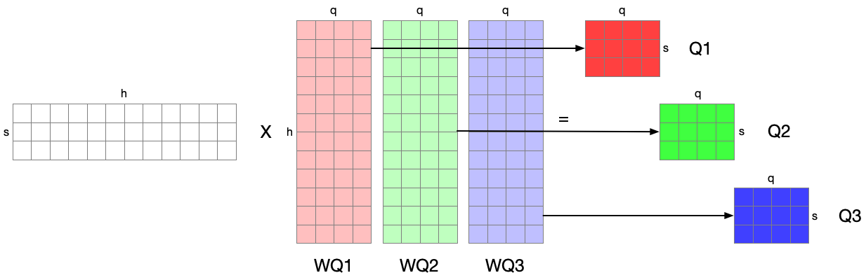
From: [$s, h$] * [$h, h$] = [$s, h$] $\rightarrow$ To: $a$ independent linear [$s, h$] * [$h, \frac{h}{a}$] = $a$[$s, \frac{h}{a}$]

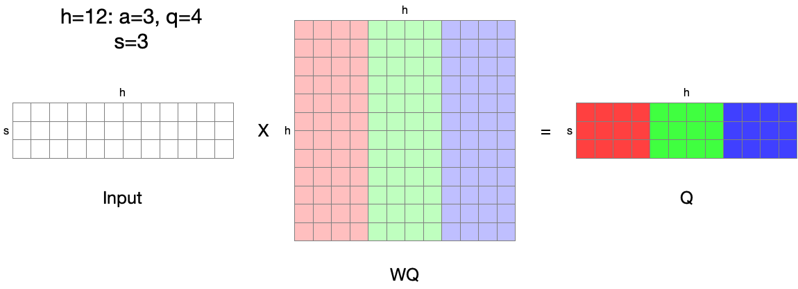
This single linear projection can be split into $a (==3)$ independent linear projections: If we say the three linear projections are distributed, no communication is needed except for the input between GPUs.

Parallelizing Attention Calculation #

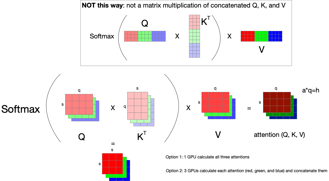
$attention(Q, K, V)=softmax(\frac{QK^T}{\sqrt{d_k}})V$

Attention calculation can also be done with concatenated Q, K, and V to calculate multi-head attentions at once, or independently calculate each attention with split Q, K, and V. But note, that Q, K, and V are not used as concatenated for matrix multiplication; each $Q_i$, $K_i$, and $V_i$ should be used independently for each attention calculation. To be specific, it is not a simple matrix multiplication of [$s, h$] $\times$ [$h, s$] $\times$ [$s, h$], but $a \times$ [$s, \frac{h}{a}$] $\times$ [$\frac{h}{s}, s$] $\times$ [$s, h$].

Megatron-LM uses 3D matrix multiplication to calculate attention [src]:

class CoreAttention(MegatronModule):
    ...
    def forward(...):
        # preallocting input tensor: [b * n, sq, sk]
        matmul_input_buffer = get_global_memory_buffer().get_tensor(
            (output_size[0]*output_size[1], output_size[2], output_size[3]),
            query_layer.dtype, "mpu")

        # Raw attention scores. [b * n, sq, sk]
        matmul_result = torch.baddbmm(
            matmul_input_buffer,
            query_layer.transpose(0, 1),   # [b * np, sq, hn]
            key_layer.transpose(0, 1).transpose(1, 2),  # [b * np, hn, sk]
            beta=0.0, alpha=(1.0/self.norm_factor))

torch.baddbmm(input, batch1, batch2, *, beta=1, alpha=1, out=None) -> Tensor

torch.baddbmm performs a batch matrix-matrix product (or matrix multiplication with broadcasting); so if batch1 is $(b \times n \times m)$ and batch2 is $(b \times m \times p)$, the input and output dimension is $(b \times n \times p)$ (first dimension $b$ is broadcasted to $(n \times m) \times (m \times p)$ matrix multiplication).

Therefore, by simply adjusting the first dimension to specify how many attentions should be computed together, attention calculation can easily be parallelized. In the example above, if we have 3 attention heads ($a=3$) and 3 GPUs, we can distribute one attention calculation to each GPU by setting the first dimension to 1.

Parallelizing Feed Forward Network (MLP) #

MLP layer includes two linear projections and GeLU; it can be expressed as follows (definition from the Attention paper ³):

$FFN(x) = max(0, xW_1 + b_1)W_2 + b_2$

where the dimension of $x$ is [$s, h$], $W_1$ is [$h, 4h$], $W_2$ is [$4h, h$].

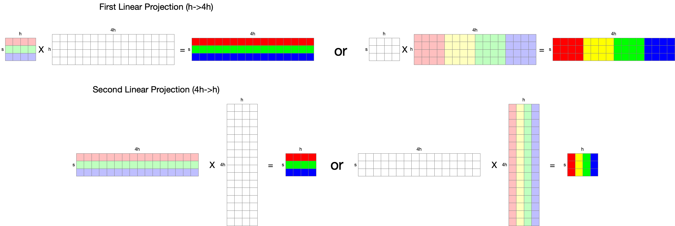
There are two ways of parallelization: split input in a row-parallel manner (left), or split weight in a column-parallel manner (right). Considering that we need to perform the second linear projection with the output of the first linear projection after GeLU applied (element-wise operation), applying row-parallelization is reasonable, since it does not require communication across nodes if they already have a replicated weights. If we apply column-parallelization for the first linear projection, data should be exchanged in nodes (either every node has a replication or at least a row).