Table of Contents

Distributed deep learning refers to use a distributed system that includes several workers to perform inference or training deep learning. Since mid 2010, people have been thinking about accelerating deep learning with scale-out, and distributd deep learning has been introduced. Parameter server is one of the well-known architecture for distributed deep learning.

Recent days, many parallelization mechanisms, the way of distributing computation to multiple workers, have been introduced. First one was to split batches into several microbatches and distributed it, namely data parallelism, which the parameter server architecture is for. But there are more parallelisms that are being used: tensor parallelism, and (pipeline) model parallelism.

This post introduces such three types of parallelism: data parallelism, tensor parallelism, and pipeline parallelism. For clear understanding, I use the following terms across the post:

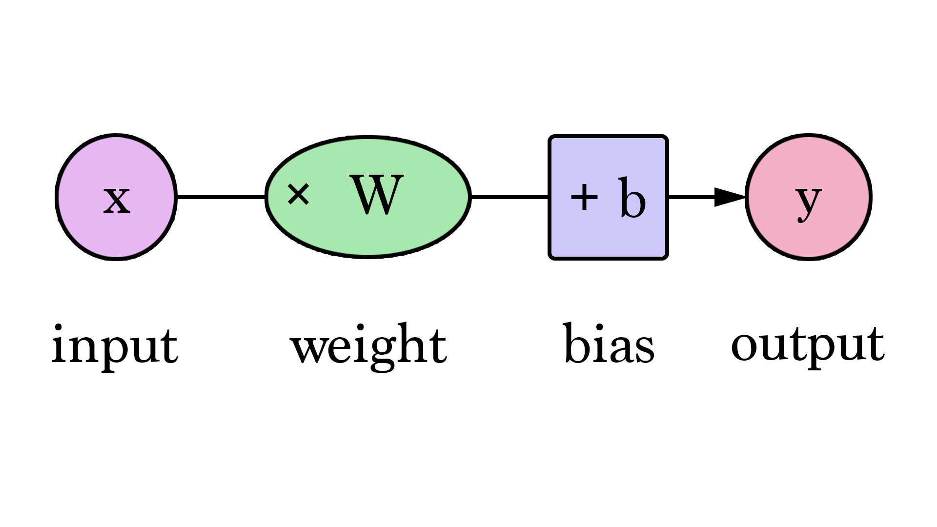
Parameters: model layer’s weights.
Output: results of forward pass.
Gradients: results of backward propagation.

Simple neural network layer example. [Source]

Data Parallelism #

Data parallelism refers to parallelism that slices a big batch into several microbatches, and distributed it into the workers.

We have to increase batch size to increase accelerator utilization, however, it might not fit into accelerator’s memory due to large amount of inputs and computed outputs. Data parallelism is based on this observation; by slicing batch by N, each accelerator would only handles 1/N inputs and only generates 1/N outputs.

With data parallelism, parameters (weight) are replicated to all accelerators, and all of them performs the same computation.
If training is done with synchronous stochastic gradient (SGD), backpropagation results or gradients should be aggregated and parameters should be updated. We can use parameter server architecture, or recently introduced all-reduce by Baidu can also be used.
If total batch size (or global batch size) is too large, it may affect the convergence rate ¹. Hence, data parallelism cannot be used for infinite scale-out.

Parameter Server #

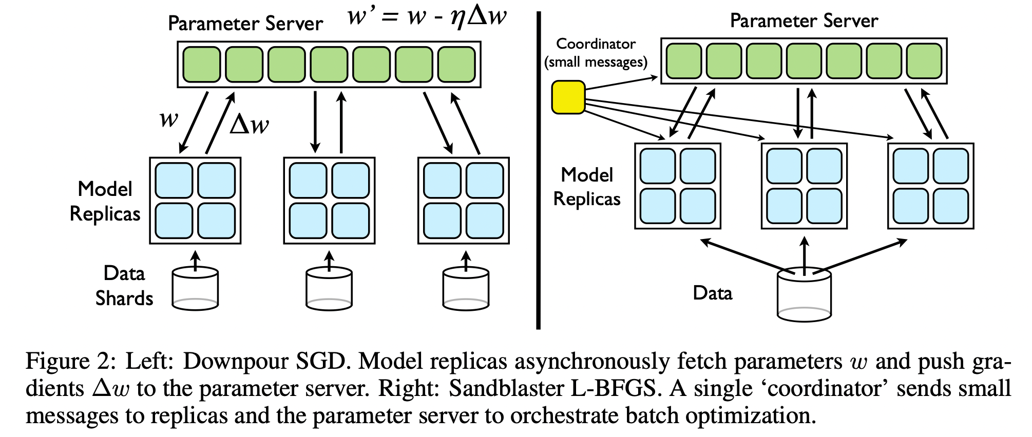
Parameter server is developed by Google and introduced in their DistBelief paper² published in NIPS 2012. It is a very famous architecture for data parallelism.

All-Reduce #

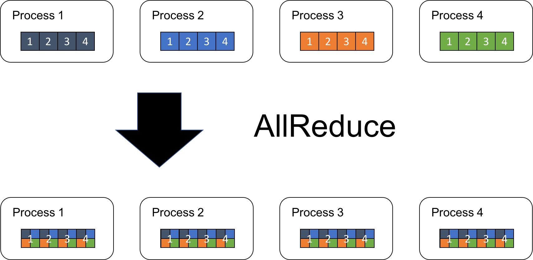
As the number of parameters grow, parameter server becomes bottleneck, making high performance accelerators under-utilized. Baidu brung ring-based all-reduce algorithm into distributed machine learning area; such collective communication came from MPI field³. The idea is to perform updates without using centralized server, by communicating directly with each other accelerators.

Refer to the reference blog ³ for more detail.

All-reduce operation can be decomposed and implemented with reduce-scatter and all-gather, other MPI techniques in HPC field ⁴. NVIDIA Collective Communication Library (NCCL) includes this version of implementation, in a ring-based manner.

Collective communication algorithms have been analyzed for decades, and this paper is one of those ⁵ (Section 2.3). For instance, the cost of operation can be modeled by $A \times \alpha + B \times N \beta + C \times N \gamma$, where $\alpha$ is the time for a message be transferred (imagine sending a 0 byte message; it should be transferred through some medium), $\beta$ is the time to process one byte of data, and $\gamma$ is the cost to perform the reduction operation per byte, and N is the size of message. Each factor is called latency ($A \times \alpha$), bandwidth ($B \times N \beta$), and computation factor ($C \times N \gamma$), respectively.

For ring based all-reduce operation, factors are as follows:

latency factor: $2(p-1) \alpha$
bandwidth factor: $2 \frac{p-1}{p}N \beta$
computation factor: $\frac{p-1}{p}N \gamma$

where $p$ is the number of processes.

Explaination: if we have $p$ numer of processes, each data should be partitioned into $p$ chunks, the size of each of which is $\frac{N}{p}$, and $p-1$ data exchange should happen. There are two (send and receive) messages involved for each data exchange, so latency factor is $2(p-1)$.

Data is transferred using a logical ring communication pattern, namely $p_0 \rightarrow p_1 \rightarrow … \rightarrow p_{p-1} \rightarrow p_p$. The reduce-scatter operation performs such logical ring communication pattern in $p-1$ iterations, making bandwidth factor $(p-1) \times \frac{N}{p} = \frac{p-1}{p}N$ for reduce-scatter operation. Following all-gather operation also transfers data across the logical ring, the amount of data to be transferred is the same with reduce-scatter. Hence, overall bandwidth factor becomes $2 \times \frac{p-1}{p}N$.

Tensor Parallelism ⁶ #

Tensor parallelism and pipeline model parallelism can be grouped as model parallelism, since it slices models into smaller chunks. While pipeline model parallelism distributes layers in a model, tensor parallelism slices each layer and distributes the chunks into multiple accelerators.

It is also called intra-layer model parallelism, because it is a type of model parallelism within a layer by slicing parameters.

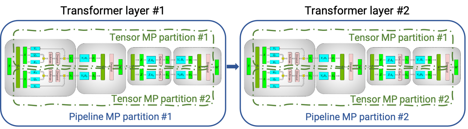
Illustration of tensor model parallel partition from Megatron-LM. [Source]

Megatron-LM is an example paper that describes such tensor parallelism. You can see that a transformer layer has been sliced to two half chunk with tensor partitioning, which can be distributed to two accelerators.

Tensor parallelism could be a good alternative to data parallelism to avoid inefficient large batch size problem, and can be used together.
Unlike data parallelism that all accelerators need to have replicated parameters, parameters are distributed along with input in tensor parallelism.
Tensor parallelism and data parallelism can be grouped as intra-layer parallelism, since they slice a tensor into multiple chunks, without affecting other layers. Imagine image classification training, whether the input tensor is 4D (width * height * color depth * batch, e.g. for ResNet: 224 * 224 * 3 * 1024 if batch is 1024). Slicing batch dimension is data parallelism (e.g. each of 4 accelerator handles 256 batches), and slicing width or height dimension is tensor parallelism (e.g. each of 4 accelerator handles 112 * 112 * 3 input).

Pipeline Model Parallelism ⁶ #

Pipeline parallelism has been introduced by Google to reduce underutilization from layer model parallelism.

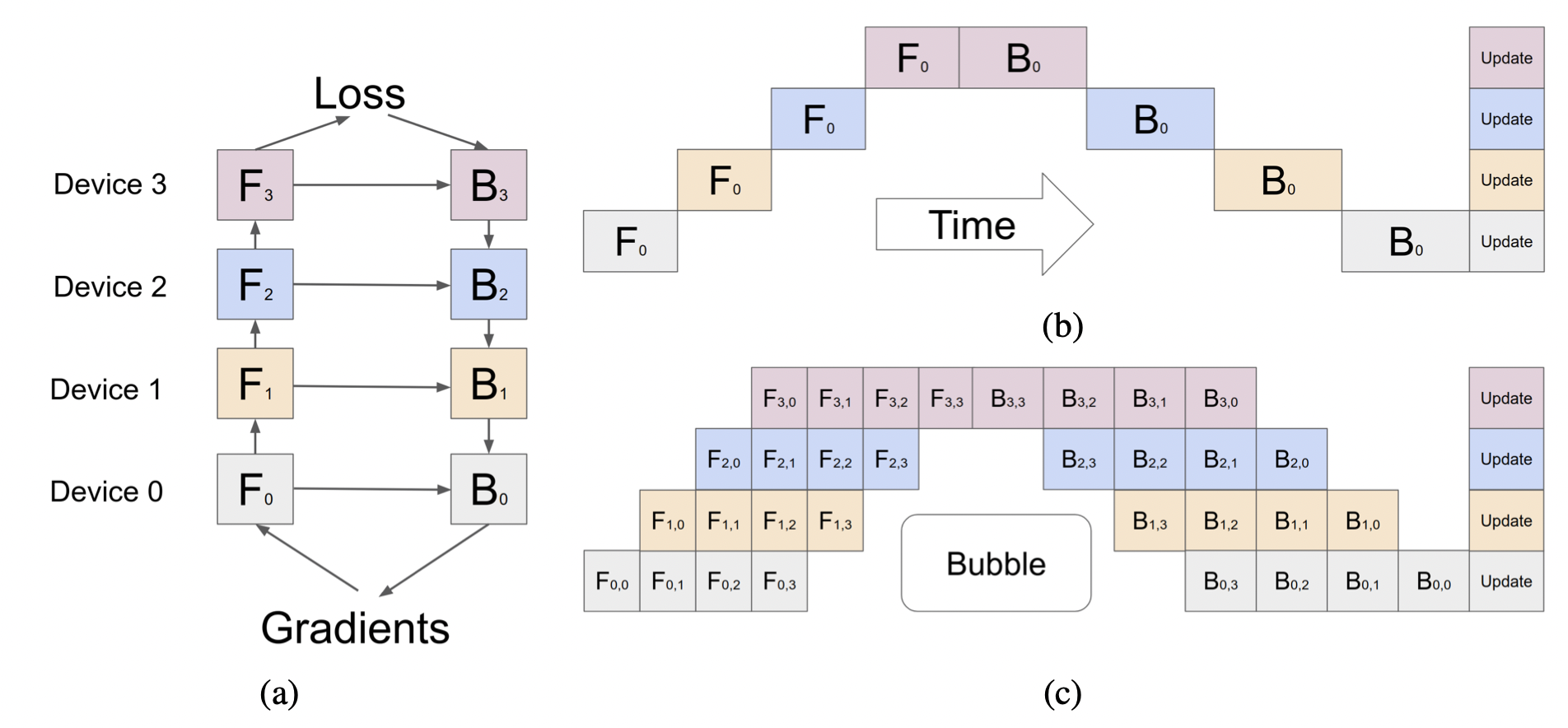
Illustration of pipeline model parallelism from GPipe. [Source]

Model parallelism means that, a model is splitted into several groups of layers (or stages), and each accelerator handles one stage (Figure (b)). It effectively reduces memory usage of each accelerator, however, it has critical drawback: all but one accelerators are idle at a time. GPipe mitigates this underutilization issue by adopting pipeline; it divides a batch into smaller micro-batches (e.g. $F_{0,0}, F_{0,1}$), and perform model parallelism independently for each micro-batch input.

The underutilized area is called bubble, and more recent works for less bubble include Pipedream (SOSP19): use asynchronous gradient update, DAPPLE (PPoPP21), and Chiemra (SC21): adopt replicated bidirectional pipeline ⁷ ⁸ ⁹.

Pipeline parallelism, unlike the former two, is inter-layer parallelism; it distributes whole layers into multiple accelerators.
For this reason, Alpa (OSDI22) re-organize parallelism into intra-OP parallelism (data+tensor) and inter-OP parallelism (pipeline) ¹⁰.
By its nature, pipeline parallelism cannot achieve 100% utilization. But 3d parallelism formulates that 81% and 90% utilization can be achieve with the number of micro-batches 4x or 8x the number of pipeline stages ¹¹.

Hybrid Parallelism #

Recently, more papers are focusing on combining all of these parallelism, namely hybrid parallelism, to support bigger training model more efficiently.